On two-dimensional qualitative LMs for gene expression analysis
When dealing with differential gene expression analyses (DEAs), one can often come across a difficulty of interpreting the linear models that are used to detect differentially expressed genes, especially when more than one experimental variable is considered.
Both the limma and DESeq2 packages are very famous packages for running DEAs. They both
use linear models (LMs) - generalized linear models (GLMs) for DESeq2- to
model the expression of every gene across all considered conditions, and use
the associated p-values and beta coefficients of the resulting models to detect
DEGs.
The simplest case is when a single variable, x, is used in the model. Simpler
still if this variable is qualitative (a factor() in R).
For instance, one might be interested in the differences between normal cells
(x = 0) and transformed cells (x = 1).
We would assume, then, that every gene $\eta$ is expressed as a function of x in this form:
$$ Y_\eta = \beta_0 + \beta_1 X_\eta $$
Where $Y_\eta$ is the expression of the gene and $X_\eta$ is the variable of interest. The realization of $Y_\eta$, $y_\eta$ is the actual estimated expression value of the gene $\eta$ given some realization $x_\eta$.
If $X_\eta$ is a binary qualitative variable, then the possible realizations $x_\eta$ can only be two. The choice of setting these possible values to $0$ and $1$ are completely arbitrary, and may be substituted by any other value. However, setting exactly these two possible realizations does aid in the interpretation of the model: the $\beta_1$ coefficient then becomes the effect of “turning on” the qualitative variable ($x_\eta$ stops being $0$, removing the effect of the coefficient, and becomes $1$, having to effect on the actual value of the coefficient).
The equation above can be visualized with a plot, like in the figure below, with $\beta_0 = 1$ and $\beta_1 = 1.2$:
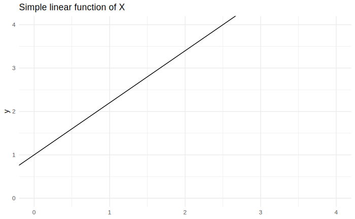
If $x$ represents a qualitative response, the only values of $y$ that make sense to consider are at $x = 0$ or $x = 1$. The domain of the linear model is $+\infty$ to $-\infty$, but keep in mind that this makes no sense in actuality. Even if $x$ was a quantitative variable, its realizations would probably not span the whole domain of the model. Always keep in mind the range of values that the model makes sense in.
In a real setting, the $\beta$ coefficients are estimated from the data, having $y$ being the expression value for that specific gene.
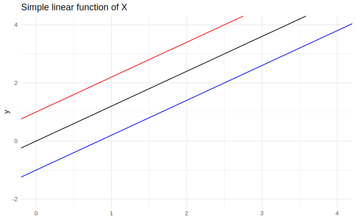
It is useful to take a moment to describe the effects of each of the coefficients: The $\beta_0$ coefficient, the intercept, has the effect of moving the function up and down, like so:
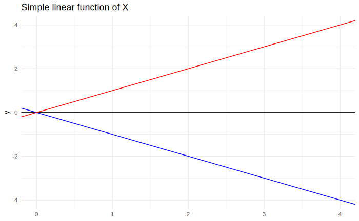
On the other hand, the value of $\beta_1$, the angular coefficient, causes the angle between the function and the $x$ axis to change, like so:
Depending on the value of $\beta_0$ and $\beta_1$, we might end up in different “scenarios”: The intercept may be positive, zero or negative, and the angular coefficient can do the same. In total, we have $3 * 3 = 9$ possible combinations:
- $\beta_0 = 0$ and $\beta_1 = 0$;
- $\beta_0 > 0$ and $\beta_1 = 0$;
- $\beta_0 < 0$ and $\beta_1 = 0$;
- $\beta_0 = 0$ and $\beta_1 > 0$;
- $\beta_0 > 0$ and $\beta_1 > 0$;
- $\beta_0 < 0$ and $\beta_1 > 0$;
- $\beta_0 = 0$ and $\beta_1 < 0$;
- $\beta_0 > 0$ and $\beta_1 < 0$;
- $\beta_0 < 0$ and $\beta_1 < 0$.
All these combinations are shown in the plot below:
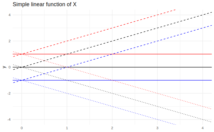
The effect of the intercept depends highly on its magnitude, but it merely translates the function around. In many settings, scientists are therefore mostly interested in the angular coefficient $\beta_1$ - which measures the magnitude of the effect - rather than $\beta_0$, so it is fair to disregard the value of $\beta_0$ not because it is unimportant, but because it is uninteresting.
The magnitude of the $\beta_1$ coefficient is also often not interesting if the $x$ variable is a dummy variable, taking the place of a qualitative variable, then the magnitude of the related $\beta$ is not important: it can be changed at will by coding the $x$ variable in different ways (e.g. instead of $x = 0$ and $x = 1$, one could use $x = -10$ and $x = +10$, making the coefficients much larger). If these dummy variables are instead coded with realizations of $0$ and $1$, then the magnitude of $\beta_1$ is interesting, as we discussed above. If the $x$ variable is instead a quantitative one, then (when chosen with an appropriate unit of measure) its magnitude is always interesting.
Having to consider the magnitude of the effects (i.e. coefficients) for every gene needs its own discussion, so we will disregard them for now.
With these considerations, we can reduce the number of “interesting” cases that we might end up with to just three, based on the sign of $\beta_0$: $\beta_0 = 0$, $\beta_0 > 0$ and $\beta_0 < 0$.
We have limited the discussion to $\beta$ coefficients, disregarding p-values. Very broadly speaking, p-values relate to how confident we are that the coefficient that they relate to is “non-zero”. If the $\beta$ coefficient has a very large p-value, we can assume that its value, for interpretation purposes, might as well be zero.
In a real regression setting, where we are presented with an estimate and related p-value for each coefficient, we can therefore fall in one of three categories:
- The p-value is significant for some $\alpha$, and $\beta > 0$;
- The p-value is significant for some $\alpha$, and $\beta < 0$;
- The p-value is not significant for some $\alpha$.
From now on we will assume that our $\alpha$ error is set to $0.05$, so when we say that a coefficient is “significant”, we mean that its related p-value is strictly less than $0.05$.
It might be important to also set a boundary to the value of $\beta$ to be sufficiently high to not fall in the same category as those beta coefficients that are not significant. With many observations, even tiny effects can become significant. However, this might not mean that they have a large enough effect to be relevant in the real world. We could then set some threshold $k$ for which our three scenarios become:
- The p-value is significant for some $\alpha$, and $\beta > k$;
- The p-value is significant for some $\alpha$, and $\beta < -k$;
- The p-value is not significant for some $\alpha$ or $-k >= \beta <= k$.
Notice how the expression of a gene can never be below zero. That means that, to fall in the “significant p-value + $\beta_1 < 0$” category, it means that $\beta_0$ must be greater than zero.
The most important things to keep in mind are that:
- For interpretation purposes, the intercept is often not important;
- If a p-value related to a coefficient is not significant, it has the same interpretation as it being zero;
- A simple linear model of the type $y = \beta_0 + \beta_1x$ can fall into one of three “interesting” categories, depending on the combination of p-value and sign of the $\beta_1$ coefficient.
To exemplify these notions, imagine a gene that is modeled by a simple formula $expr = \beta_0 + \beta_1x$, where $x$ is a dummy factorial variable of $x = 1$ if the sample is a transformed cell and $x = 0$ if the sample is a normal cell. Let’s relate each possible case that we might fall in to its interpretation:
- A non-significant $\beta_1$: in this case, the gene does not vary due to the experimental condition $x$;
- A significant $\beta_1 > 0$: in this case, the experimental condition $x$ causes an increased expression of the gene. This is a “canonical” up-regulated DEG.;
- A significant $\beta_1 < 0$: in this case, the experimental condition $x$ causes a reduced expression of the gene. This is a “canonical” down-regulated DEG.
Additionally, in this particular case, the magnitude $\beta_1 > 0$ or $\beta_1 < 0$ is the actual fold-change difference between the expression of the gene is the normal vs tumor samples. This is why DESeQ2 calls
fold_changethe column that actually holds the $\beta$ coefficient values.
Adding one more variable
If we have to consider two experimental variables, $x_1$ and $x_2$, we start to be faced with additional challenges.
It is best to start by considering the two variables as different models. A possible visualization is:
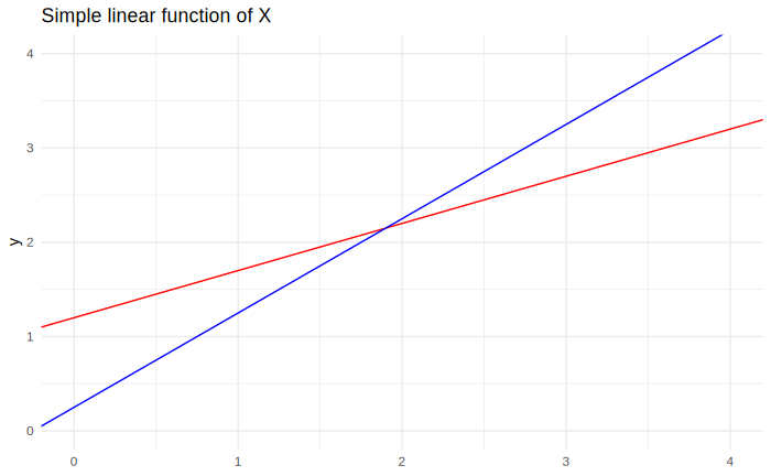
In this exemplification, we have two lines:
$$ y = \beta_0^1 + \beta_1^1x_1 $$ and $$ y = \beta_0^2 + \beta_1^2x_2 $$
Imagine that, in this case, the $\beta$ coefficients are estimated from the data. All the considerations made before hold, independently, for both models. The models are non constrained by each other in any way.
Another possible representation of the same two, independent models is in 3D space: in this space, the $y$ axis is vertical, the $x_1$ axis is horizontal, and the $x_2$ axis is perpendicular to the other two. If we plot the two functions above in such a space, we will get the following:
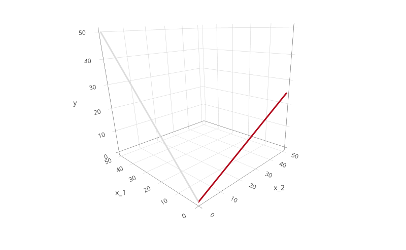
Here, the two models lay on the $y, x_1$ and $y, x_2$ planes. They are completely independent of each other: the representation is the same as the two lines in the plot above, but each on their own plane.
However, we want to consider our two variables together. To do this, we can write the following model: $$ y = \beta_0 + \beta_1x_1 + \beta_2x_2 $$
Such a model takes into account the effects of both variables when estimating $y$, exactly what we want. This results in the following plot:
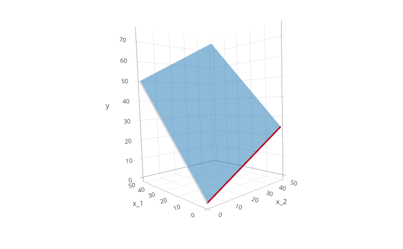
The two lines from the above plot are drawn in this plot too. As you can see, the model now describes a plane. The plane intersects the $y, x_1$ plane (where $x_2 = 0$) at exactly $y = \beta_0 + \beta_1x_1$. In the same way, the plane intersects the $y, x_2$ plane (where $x_1 = 0$) at exactly $y = \beta_0 + \beta_2x_2$. This tells us that the two simple models above are actually contained in this, more complex model.
Note that the $beta_0$ coefficient was set to $0$ in all example plots for simplicity, but it may change between the separated and “combined” models in practice. However, it always intercepts the plane similar to these simple examples.
We can make an important observation: the plane, no matter the $\beta$ coefficients, can only be perfectly flat. This is easy to understand: when “rising” from the $x_1$ axis (as $x_2$ increases), the plane can only vary by a fixed amount, $\beta_2$. The same holds when looking at the $x_2$ axis, the plane can only vary by the fixed amount governed by $\beta_1$.
However, we might be in a situation where the two variables interact. This means that the $\beta_1$ coefficient could vary based on the value of $x_2$, or vice-versa. This property can be taken into account by introducing an interaction term in the model: $$ y = \beta_0 + \beta_1x_1 + \beta_2x_2 + \beta_3x_1x_2 $$
The interaction term $\beta_3x_1x_2$ causes a particular change in the resulting plane: it allows it to bend.
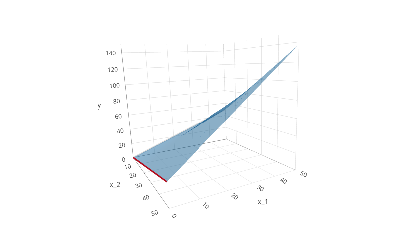
This new “bent” plane takes into account the (possible) synergy (or antagonistic effect) between $x_1$ and $x_2$.
This might seem far-fetched when considering gene expression, but it turns out that it is not. Many experimental models take into account two experimental variables, often generating all samples that cover all their possible combinations.
Since an interaction between the two variables cannot be ruled out a priori (we cannot rule out a “bent” plane), an interaction term is needed in these situations to model the expression of each gene.
I hypothesize that, even if the interaction term is not significant in all genes (or just a handful of them), it would be wrong to remove the interaction term altogether, as the samples do vary in both dimensions, and a non-significance does not mean necessarily no interaction of the variables, just that, if it is there, we cannot detect it.
A problem arises when one needs to interpret such a model. However, we can use a similar approach as with the simple linear model. In this case, however, our degrees of freedom are higher, so there are more possibilities to explore. We can keep in mind:
- We are only considering the (narrow) case where $x_1$ and $x_2$ are independent dummy variables that take the values of $0$ and $1$.
- We disregard, for the same reasons above, the value of the intercept, $\beta_0$.
- We can use the p-value considerations made for simple models to “collapse” all possible $\beta$ values to just three categories (positive, negative or non-significant/zero).
Keeping this in mind, our search space becomes manageable. We need to interpret $3 \cdot 3 \cdot 3 = 27$ separate cases:
- If $\beta_3 = 0$:
- (1) $\beta_1 = 0$ and $\beta_2 = 0$: There is no evidence of any effect of the conditions on the expression of the gene;
- (2) $\beta_1 > 0$ and $\beta_2 = 0$: There is evidence of an increased expression of the gene under the $x_1$ condition, which is seemingly independent of $x_2$. There is no evidence of any effect of the $x_2$ condition;
- (3) $\beta_1 < 0$ and $\beta_2 = 0$: There is evidence of a decreased expression of the gene under the $x_1$ condition, which is seemingly independent of $x_2$. There is no evidence of any effect of the $x_2$ condition;
- (4) $\beta_1 = 0$ and $\beta_2 > 0$: There is evidence of an increased expression of the gene under the $x_2$ condition, which is seemingly independent of $x_1$. There is no evidence of any effect of the $x_1$ condition;
- (5) $\beta_1 > 0$ and $\beta_2 > 0$: There is evidence of increased expression of the gene in both conditions, with no apparent synergistic effect;
- (6) $\beta_1 < 0$ and $\beta_2 > 0$: There is evidence of an increased expression under the $x_2$ condition, and evidence of a decreased expression under the $x_1$ condition, with no apparent antagonistic effect.;
- (7) $\beta_1 = 0$ and $\beta_2 < 0$: There is evidence of a decreased expression of the gene under the $x_2$ condition, which is seemingly independent of $x_1$. There is no evidence of any effect of the $x_1$ condition;
- (8) $\beta_1 > 0$ and $\beta_2 < 0$: There is evidence of an increased expression under the $x_1$ condition, and evidence of a decreased expression under the $x_2$ condition, with no apparent antagonistic effect;
- (9) $\beta_1 < 0$ and $\beta_2 < 0$: There is evidence of decreased expression of the gene in both conditions, with no apparent synergistic effect;
- If $\beta_3 > 0$:
- (10) $\beta_1 = 0$ and $\beta_2 = 0$: There is evidence of a positive synergistic effect between the conditions, while there is no evidence of any individual effect;
- (11) $\beta_1 > 0$ and $\beta_2 = 0$: There is evidence of a positive effect of the $x_1$ condition, while the $x_2$ condition has seemingly no effect. However, the two combined conditions cause a more pronounced positive overall effect;
- (12) $\beta_1 < 0$ and $\beta_2 = 0$: There is evidence of a down regulation caused by the $x_1$ condition, while - alone - the $x_2$ condition has seemingly no effect. However, when combined, the overall effect is [[positive/neutral/less negative, depending on $\beta_1 - \beta_3$. Unsure if the subtraction can be done, however…]];
- (13) $\beta_1 = 0$ and $\beta_2 > 0$: There is evidence of a positive effect of the $x_2$ condition, while the $x_1$ condition has seemingly no effect. However, the two combined conditions cause a more pronounced positive overall effect ;
- (14) $\beta_1 > 0$ and $\beta_2 > 0$: There is evidence that both $x_1$ and $x_2$ positively up-regulate the expression of the gene. Additionally, their effect shows positive synergy;
- (15) $\beta_1 < 0$ and $\beta_2 > 0$: There is evidence of a negative effect of $x_1$ and a positive effect of $x_2$. The interaction of these two conditions is synergically positive, [[with undefined combined outcome, depending on $\beta_1 + \beta_2 + \beta_3$]];
- (16) $\beta_1 = 0$ and $\beta_2 < 0$: There is evidence of a down regulation caused by the $x_2$ condition, while - alone - the $x_1$ condition has seemingly no effect. However, when combined, the overall effect is [[positive/neutral/less negative, depending on $\beta_2 - \beta_3$. Unsure if the subtraction can be done, however…]];
- (17) $\beta_1 > 0$ and $\beta_2 < 0$: There is evidence of a negative effect of $x_2$ and a positive effect of $x_1$. The interaction of these two conditions is synergically positive, [[with undefined combined outcome, depending on $\beta_1 + \beta_2 + \beta_3$]];
- (18) $\beta_1 < 0$ and $\beta_2 < 0$: There is evidence that both $x_1$ and $x_2$ down-regulate the expression of the gene. However, when both conditions are present, the overall effect is [[positive/neutral/less negative, depending on $\beta_1 + \beta_2 - \beta_3$. Unsure if the subtraction can be done, however…]];
- If $\beta_3 < 0$:
- (19) $\beta_1 = 0$ and $\beta_2 = 0$: There is evidence of a negative synergistic effect between the conditions, while there is no evidence of any individual effect;
- (20) $\beta_1 > 0$ and $\beta_2 = 0$: There is evidence of a positive effect of the $x_1$ condition, while the $x_2$ condition has seemingly no effect. However, the two combined conditions cause a [[negative/neutral/less positive, depending on $\beta_1 - \beta_3$]] overall effect;
- (21) $\beta_1 < 0$ and $\beta_2 = 0$: There is evidence of a negative effect of the $x_1$ condition, while the $x_2$ condition has seemingly no effect. However, the two combined conditions cause a more pronounced negative overall effect;
- (22) $\beta_1 = 0$ and $\beta_2 > 0$: There is evidence of a positive effect of the $x_2$ condition, while the $x_1$ condition has seemingly no effect. However, the two combined conditions cause a [[negative/neutral/less positive, depending on $\beta_2 - \beta_3$]] overall effect;
- (23) $\beta_1 > 0$ and $\beta_2 > 0$: There is evidence that both $x_1$ and $x_2$ up-regulate the expression of the gene. However, when both conditions are present, the overall effect is [[negative/neutral/less positive, depending on $\beta_1 + \beta_2 - \beta_3$. Unsure if the subtraction can be done, however…]];
- (24) $\beta_1 < 0$ and $\beta_2 > 0$: There is evidence of a negative effect of $x_1$ and a positive effect of $x_2$. However, when both conditions are present, the overall effect is [[negative/neutral/less positive, depending on $\beta_1 + \beta_2 - \beta_3$. Unsure if the subtraction can be done, however…]];
- (25) $\beta_1 = 0$ and $\beta_2 < 0$: There is evidence of a negative effect of the $x_2$ condition, while the $x_1$ condition has seemingly no effect. However, the two combined conditions cause a more pronounced negative overall effect;
- (26) $\beta_1 > 0$ and $\beta_2 < 0$: There is evidence of a negative effect of $x_2$ and a positive effect of $x_1$. However, when both conditions are present, the overall effect is [[negative/neutral/less positive, depending on $\beta_1 + \beta_2 - \beta_3$. Unsure if the subtraction can be done, however…]];
- (27) $\beta_1 < 0$ and $\beta_2 < 0$: There is evidence that both $x_1$ and $x_2$ down-regulate the expression of the gene. Additionally, their effect shows positive synergy, exacerbating the down-regulation further;
Those are a lot of cases! Each of our genes may fall into one of these $27$ categories, and can therefore be interpreted.
The reader can imagine that interpreting a model with three or more variables, with interaction terms, is very, very difficult. However, this method can in theory be applied to any number of variables.